How to actually train Lagrangian Neural Networks in a stable way? (Including for General Relativistic settings)

LNNs are really hard to train for systems that are not very simple. In this blog, we will explore why they are unstable, and then regularize and make some small changes to the LNN framework so that we can use it for more complex and general-relativistic systems and predict their Lagrangians.

This follows our paper, Learning Relativistic Geodesics and Chaotic Dynamics via Stabilized Lagrangian Neural Networks with Asst. Prof. Arkadaş Özakın, and our subsequent projects, Solving Schwarzschild Geodesic Motion with Lagrangian Neural Networks and Recovering Irreducible Three-Body Interactions with Lagrangian Neural Networks, by Şükrü Çağlar, and Sena Kalabalık respectively, as the AI for Theoretical Physics research group at Boğaziçi University.

We presented these projects at EuCAIFCon 2026 at Heidelberg University. You can see the conference entries for the stabilized LNN, three-body, and Schwarzschild projects if you are interested.

A quick review of LNNs

First, let’s do a quick review of LNNs. Suppose we have only trajectory data, meaning that we have a set of generalized positions, velocities, and accelerations.

LNN architecture and supervision flow.⁴

LNNs simulate this by having a neural network that takes the positions and velocities as inputs and outputs a Lagrangian. From this Lagrangian expression, using automatic differentiation, you can define the acceleration using the Euler–Lagrange equation:

$$\frac{d}{dt}\frac{\partial \mathcal L}{\partial \dot q}-\frac{\partial \mathcal L}{\partial q}=0$$

The vectorized form is

$$\ddot{\mathbf q}=M^{-1}\!\left[\nabla_{\mathbf q}\mathcal L-\left(\nabla_{\mathbf q}\nabla_{\dot{\mathbf q}}^{\!\top}\mathcal L\right)\dot{\mathbf q}\right], \qquad M=\nabla_{\dot{\mathbf q}}\nabla_{\dot{\mathbf q}}^{\!\top}\mathcal L.$$

The network learns the Lagrangian by minimizing the difference between the predicted acceleration and the real one. In other words, the network tweaks the Lagrangian to match the accelerations. This approach has advantages such as better conservation of energy. Learning the Lagrangian itself is also very useful if you want to analyze the physical system underneath it.

This blog, written by Sam Greydanus, one of the original authors of the LNN paper and the main author of the Hamiltonian Neural Networks paper, is also a great learning resource.

An inherent source of instability

Both the acceleration and the gradient updates have a factor of the inverse of the mass matrix, which is the Hessian of the Lagrangian. If our network has mass-matrix determinants close to zero, the system will become very unstable.

$$\det M\to0 \quad\Longrightarrow\quad \lVert M^{-1}\rVert\to\infty \quad\Longrightarrow\quad \text{accelerations and gradients explode.}$$

This is the main reason why the plain version of this network is really unusable when you are trying to apply it to complex systems.

The original authors, Cranmer et al., proposed a custom initialization method involving symbolic regression for the network weights to make training more stable, but that method is expensive to run and specific to the problem and the number of inputs. Even with that initialization, the performance is not where we want it to be. Liu et al. proposed a network with parallel Softplus and quadratic branches, together with an initial q̇ᵀq̇ term in the Lagrangian. We tried their full approach, but it did not stabilize our difficult systems. However, we found the initial quadratic term useful because it starts the model with a positive-semidefinite, invertible Hessian.

How can we make LNNs actually stable?

The real answer to this question is that it depends on your system of interest. For example, if you know that you are in a classical system and your coordinates are Cartesian, then you know the kinetic-energy part and can set up the Lagrangian as a known analytical kinetic-energy term plus a potential network. Even better, if you know that the potential depends only on the positions, you can give only the positions as inputs to the network. The core idea is to incorporate as much physics as possible into the network, which is common in PINN-style approaches, of which LNNs are a part.

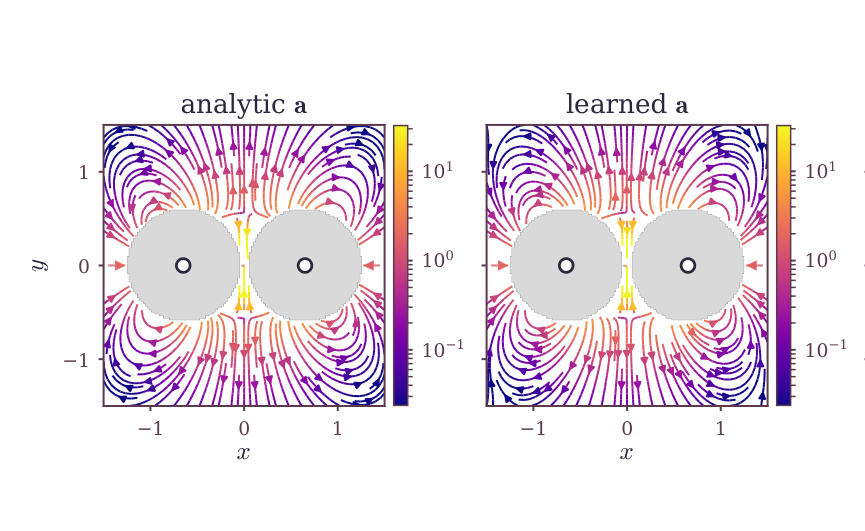
By doing these things, as well as using clever input augmentation and data-sampling techniques, we were able to train an irreducible three-body interaction Lagrangian, specifically the Axilrod–Teller potential. We even recovered an almost exact analytical version of the potential using symbolic regression, which shows that LNNs are well-suited for scientific-discovery tasks once they can be trained well!

What about the general case?

For any physical Lagrangian, we tackled this problem by regularizing the Hessian so that the loss penalizes its negative eigenvalues, which are not physical for classical systems:

$$\mathcal L_{\mathrm{eigen}} =\operatorname{MAE}(\ddot{\mathbf q}_{\rm real},\ddot{\mathbf q}_{\rm pred}) +\lambda\sum_{\lambda_i<0}|\lambda_i|.$$

This, together with smaller changes such as using GeLU activations, clipping the gradient norm at 1, applying physics-aware coordinate normalization, adding an initial quadratic velocity term, and widening the training range of periodic coordinates, makes the network much more stable. It allows us to train it for double pendulums much more reliably.

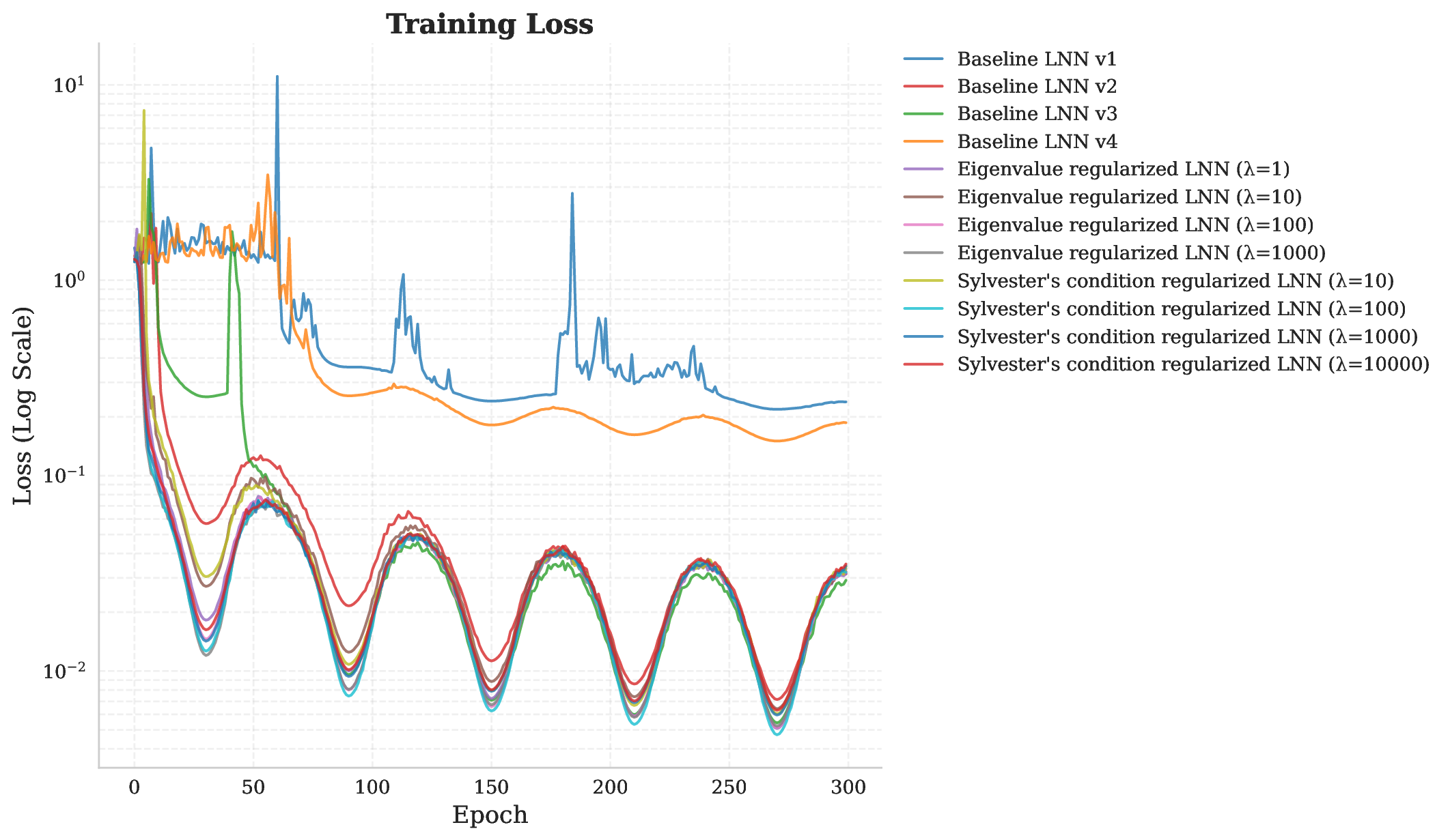
We can go further and train spring pendulums and triple pendulums as well.

Of course, these are chaotic systems, and the more relevant benchmark here is conservation of energy rather than only a pointwise prediction comparison.

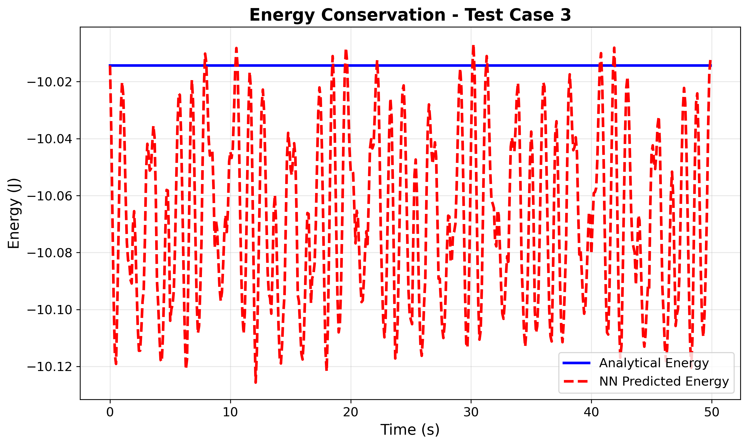
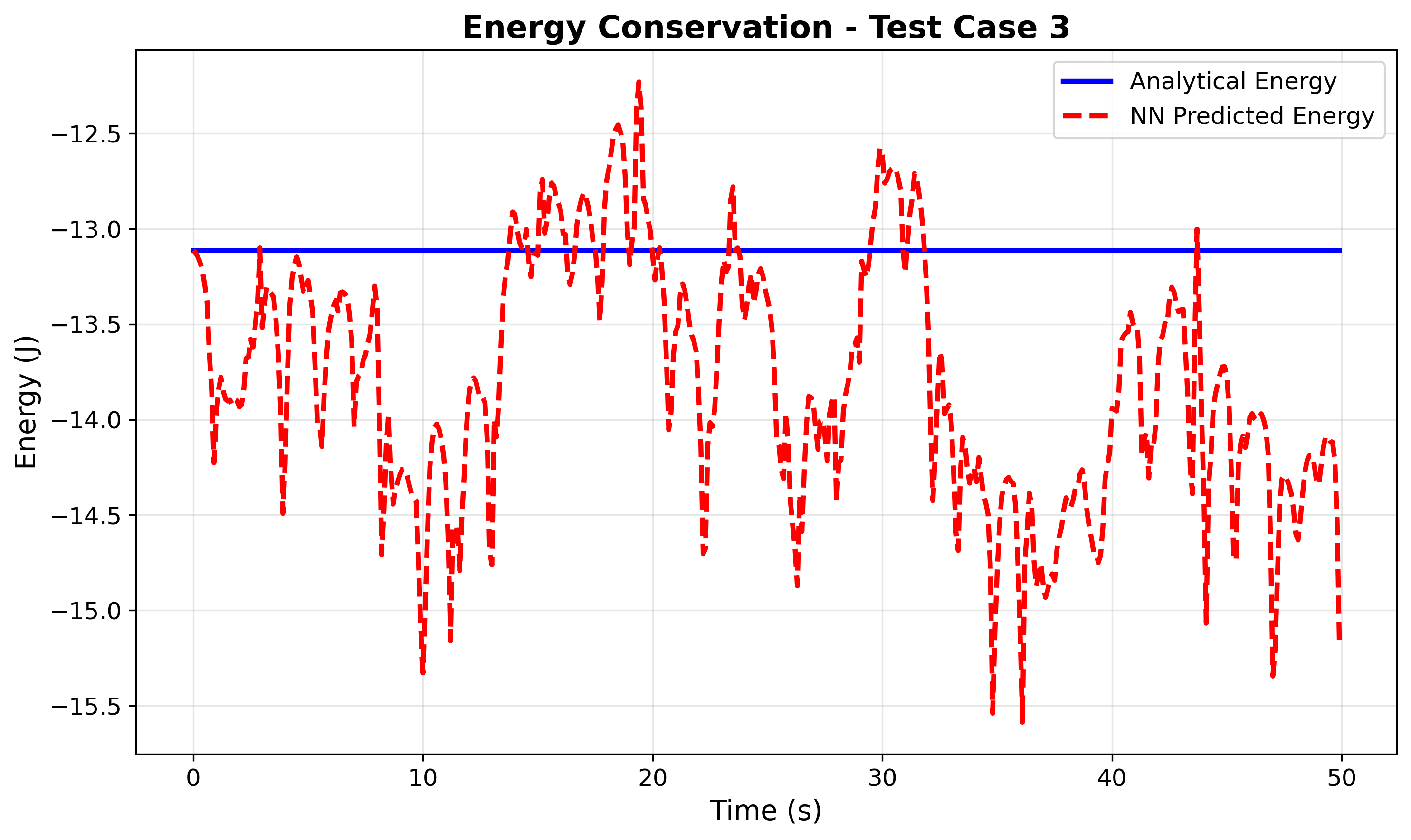
Before this regularization contribution, it was very hard for the LNN to decrease the loss enough to produce a meaningful simulation.

Using the regularized version of LNNs to solve geodesic motion

Another line of work is to give the model the motion of a particle following a geodesic, so that it can simulate the motion and learn the geometry of the system. We can write these systems using a kinetic Lagrangian that encodes the geometry of the underlying manifold.

$$\mathcal L=\frac12mR^2\left(\dot\theta^2+\sin^2\!\theta\,\dot\phi^2\right).$$

Extending LNNs to general-relativistic systems

Extending the LNN framework to general-relativistic systems means that the input becomes four-dimensional spacetime. The input also contains $t$ and $\dot t$, where the dot denotes a derivative with respect to proper time.

$$q^\mu=(t,x,y,z),\qquad \dot q^\mu=(\dot t,\dot x,\dot y,\dot z),\qquad \ddot q^\mu=(\ddot t,\ddot x,\ddot y,\ddot z).$$

The way we do this is to suppose that the region of interest has a timelike coordinate. By convention, it is at index 0. Relativistic systems have a Lorentzian signature in their Hessian, which means that the eigenvalue corresponding to the timelike coordinate needs to be negative while the rest need to be positive. We penalize violations by explicitly requiring $M_{00}$ to be negative, which is enough for the timelike part, and then use Sylvester’s condition for the spacelike submatrix, penalizing negative determinants of its leading principal minors.

$$\begin{aligned} \mathcal L_{\rm rel}=\operatorname{MAE}(\ldots)+\lambda\Bigg[ &\frac{\operatorname{ReLU}(M_{00})}{c_0+\varepsilon}\\[-1mm] &+\sum_{k=1}^{n-1}\frac{\operatorname{ReLU}\!\left(-\det M_k^{\rm spatial}\right)}{s_k^{\rm spatial}+\varepsilon} \Bigg]. \end{aligned}$$

A quick proof of concept was the AdS₄ spacetime metric, using the “half-space” coordinates analogous to the Poincaré half-space model of hyperbolic space:

$$ds^2=\frac1{z^2}\left(-dt^2+dx^2+dy^2+dz^2\right).$$

Our model successfully predicted the trajectory. We can also compare the time-dilation factor $\dot t$, which it predicted very successfully as well, although both tests cover only short periods of time.

Learning Schwarzschild geodesic motion with LNNs

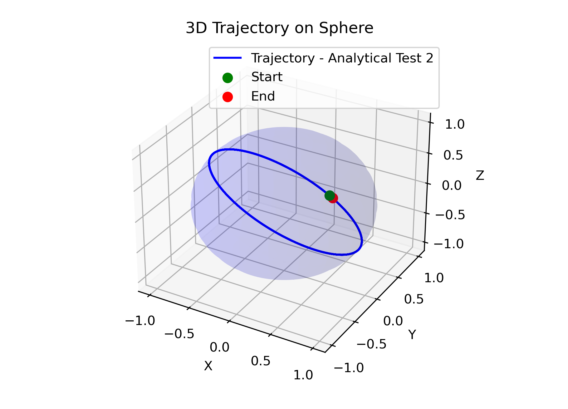
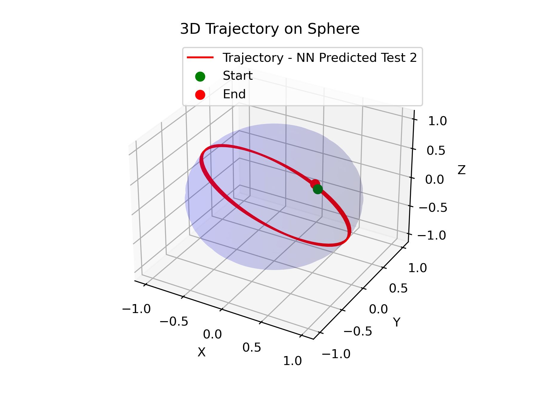
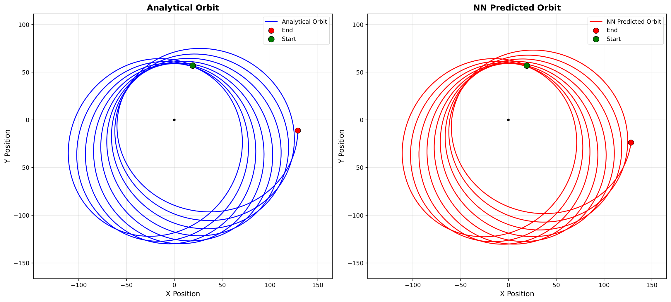
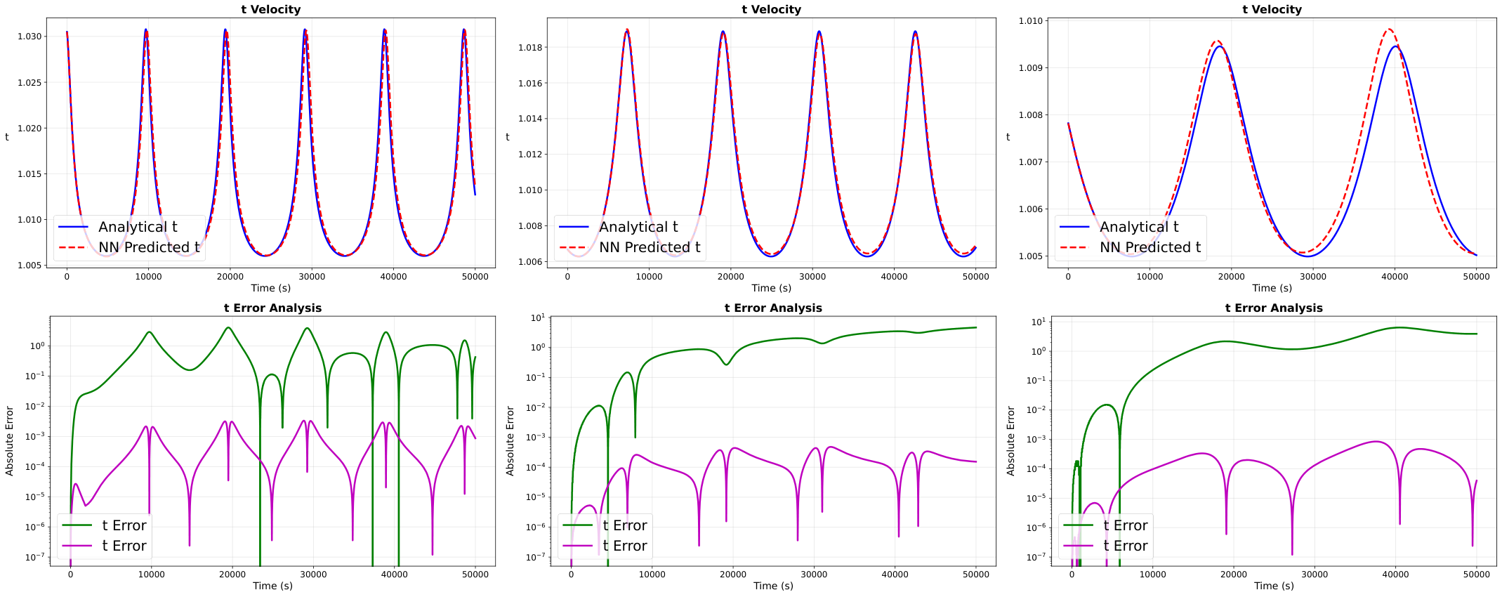
By changing the sampling strategy and adding a “decoupled” normalization to both the inputs and the accelerations, we were also able to train an LNN on Schwarzschild geodesic motion. It found the correct time-dilation factors and simulated long-horizon trajectories quite well, again using only trajectory data. This showcases a real use case that was out of reach before the changes made to the framework.

Can we recover the analytical Lagrangians and/or metric tensors with this?

Since we now have a stable way of using LNNs, can we go one step further and hope to recover analytical Lagrangians and metric tensors through automatic differentiation? Sure! But maybe not in the form that is familiar to us. The reason is simple: Lagrangians are not unique.

You might be saying, “Well, of course they are not unique; you can add any total time derivative of a function of positions to them,” which is true. Something less well known is that the gauge freedom does not end there, and there is a concept of “inequivalent Lagrangians.” The relevant inverse problem is constrained by the Helmholtz conditions, which determine whether a system of differential equations can arise from an Euler–Lagrange equation. In some cases involving geometry, inequivalent Lagrangians can be readily seen: a geodesic system with a purely kinetic Lagrangian can sometimes also be represented by a different formulation containing an effective potential.

Therefore, the recovered Lagrangians or mass-matrix elements, or metric-tensor elements in the relativistic case, do not have to look at all like what you expect. A curious result is that, for the double pendulum and various classical systems, plots of both the Hessian and the Lagrangian itself were very similar to their analytical counterparts.

This is something for which I could not find an answer: Why do they converge to the Lagrangian that we use analytically? What makes that Lagrangian special? Is it because our regularization favors it, or is it about the representational simplicity of the Lagrangian? An answer at this stage surely cannot be general, since for the Schwarzschild case the results were more different than similar, especially for the metric-tensor elements.

Future work

I believe that the methods outlined here enable many different things to be done with LNNs. One possible direction I have considered is this: Can we make our networks privilege a representation of the Lagrangian and the mass matrix that will definitely be useful to us, potentially by using the Helmholtz conditions? An example of regularizing through these conditions is Luca Wolf and collaborators’ work on discovering Euler–Lagrange equations from trajectory data.

LNNs also need good coordinates to start with, but for scientific-discovery tasks we might have only something like Cartesian coordinates. For pendulums, we might not know that there are rods, and we might not know that their lengths do not change at all. Thus, I have worked on learning holonomic constraints alongside the Lagrangian and succeeded in training such a model. If you want to learn more, you can check out this blog piece that I have also written:

Continue reading Learning both the Lagrangian and the holonomic constraints from trajectory data →

Bibliography

1. Hamzaogullari & Ozakin, Learning Relativistic Geodesics and Chaotic Dynamics via Stabilized Lagrangian Neural Networks
2. Cranmer et al., Lagrangian Neural Networks
3. Liu et al., Machine-Learning Non-Conservative Dynamics for New-Physics Detection
4. EuCAIFCon: stabilized LNNs
5. EuCAIFCon: irreducible three-body interactions
6. EuCAIFCon: Schwarzschild geodesic motion