Learning both the Lagrangian and the holonomic constraints from trajectory data

We want to simulate and also analyze physical systems. A tool that is great for both is Lagrangian Neural Networks. In this blog, I will show how to learn both the Lagrangian and the holonomic constraints of a system from trajectory data, including the number of constraints.

This project was my Bachelor’s thesis, with my advisors Dr. İnci Meliha Baytaş and Dr. Arkadaş Özakın. I also presented it at EuCAIFCon 2026 at Heidelberg, Germany. And also, if you want to learn more about Lagrangian Neural Networks, here is a blog where I gave a brief introduction to them.

Why would we want to learn constraints at all?

Lagrangian Neural Networks need to have “good generalized coordinates” beforehand to work. We have to represent the system so that the number of position coordinates is the same as the number of degrees of freedom. Take a simple pendulum, for example.

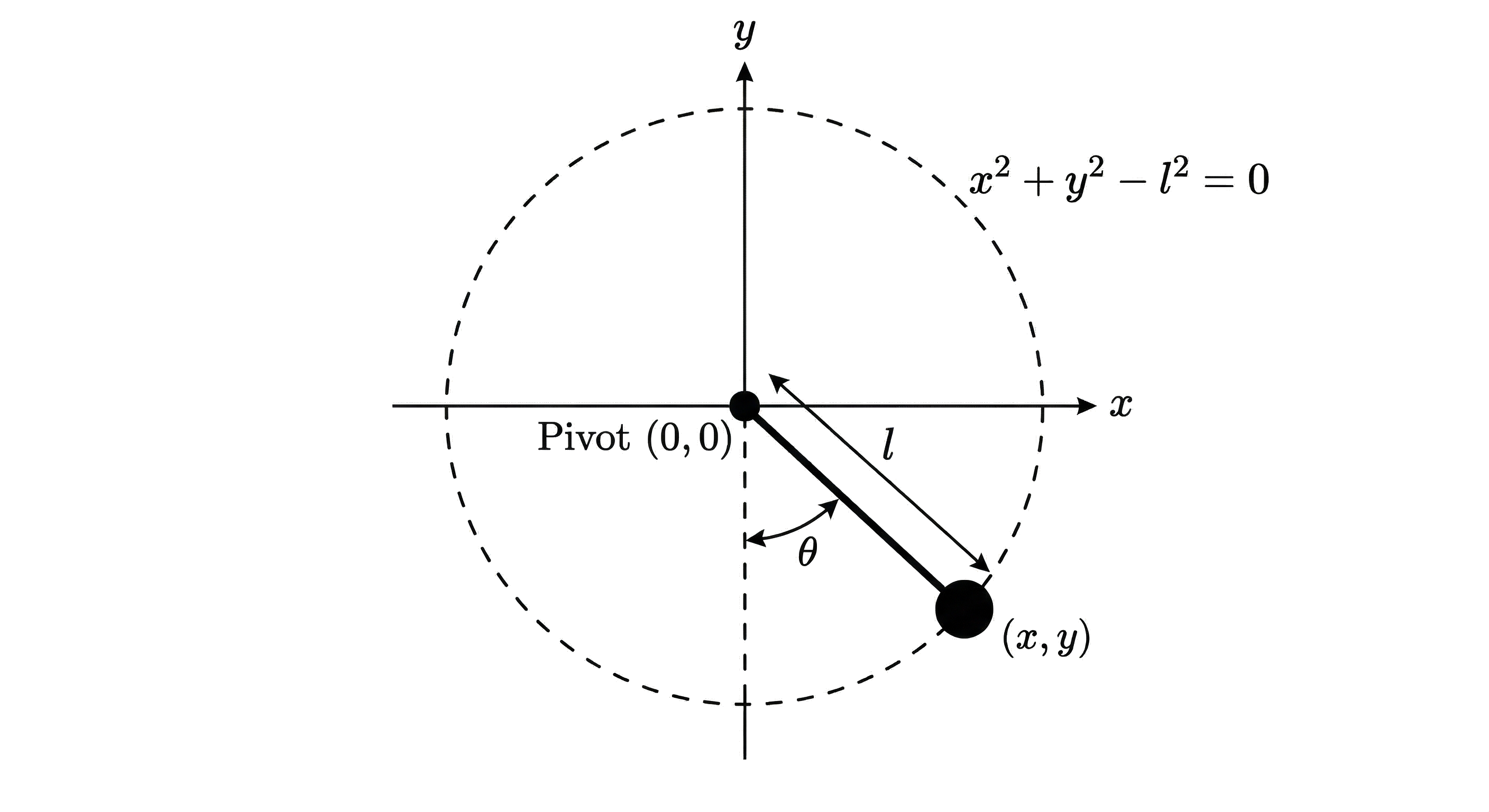
It is the angle $\theta$, in this case, that is a “good coordinate” for the system. We essentially assume that the rod length is constant and that the angle is enough to represent the system. The pendulum has the constraint

$$\phi(x,y)=x^2+y^2-\ell^2=0.$$

But in black-box scientific-discovery scenarios, we may observe only the motion of the particle in Cartesian coordinates, such as $(x,y)$, without ever knowing that there was a rod or that its length is constant.

So, given a dataset of trajectories, we want to predict the Lagrangian and the holonomic constraints of the system together, including the number of constraints, to predict the correct dynamics.

There is already some work modifying LNNs with constraints. Finzi et al.² modify Lagrangian Neural Networks to always work in Cartesian coordinates and explicitly provide the constraints. They then use the constrained Euler-Lagrange equation to solve for the acceleration:

$$\frac{d}{dt}\nabla_{\dot{\mathbf q}}\mathcal L -\nabla_{\mathbf q}\mathcal L +J^\top\boldsymbol\lambda=\mathbf 0, \qquad J=\nabla_{\mathbf q}\mathbf\Phi.$$ $$\ddot{\mathbf q}=M^{-1}\!\left[ \mathbf f+J^\top(JM^{-1}J^\top)^{-1} \left(JM^{-1}\mathbf f+\dot J\dot{\mathbf q}\right) \right], \qquad M=\nabla_{\dot{\mathbf q}}\nabla_{\dot{\mathbf q}}^{\!\top}\mathcal L.$$

They claim that it is much easier to train in Cartesian coordinates because the forms of the Lagrangians are much simpler in that case. However, there was no work in the literature that predicted both the constraints and the Lagrangian of the system at the same time, until now.

How can we learn both together?

For this, we train two separate networks: one for the Lagrangian and one for the constraints.

The joint Lagrangian and constraint-learning architecture.¹

For now, let’s assume that we know the number of constraints, so the output dimension of the constraint network is that number.

Then what? The Lagrangian has a learning signal from the acceleration, but for the constraint network, we need to add new loss terms so that it behaves like a proper constraint function.

One very intuitive term is to make the output of the learned constraint zero at the evaluated points, since our constraints are of the form $\Phi_i(\mathbf q)=0$:

$$\mathcal L_{\rm zero} =\mathbb E_i\,\|\mathbf\Phi_\psi(\mathbf q_i)\|_2^2.$$

But this has the problem of encouraging the zero function to be learned everywhere. We want only the points on the configuration manifold to be zero, but all of our samples have to be on the constraint manifold. So, we add another term, the Eikonal loss:

$$\mathcal L_{\rm eik} =\mathbb E_{i,a}\left( \|\nabla\phi_{\psi,a}(\widetilde{\mathbf q}_i)\|_2-1 \right)^2.$$

One might argue that putting this constraint on our constraint, pun intended, might break its physics. Can we just do that?

Yes, we can. Multiplying our constraints $\phi(\mathbf x)$ by an invertible function leaves the zero set intact, so it is still our constraint. The Eikonal term makes our constraint terms signed-distance functions. For the single pendulum, we can transform the constraint as

$$\phi_{\rm sdf}(x,y) =\sqrt{x^2+y^2}-\ell =\frac{x^2+y^2-\ell^2}{\sqrt{x^2+y^2}+\ell} =\frac{\phi(x,y)}{\sqrt{x^2+y^2}+\ell}.$$

The scaling is invertible near the physical circle, and the zero set stays the same.

Our constraint function is still not a proper physical constraint function. We need to add additional terms. One concerns the velocity: our velocities need to be perpendicular to the normals of the constraints. This equation can be derived from the time derivative of the zero-set condition:

$$\mathbf\Phi(\mathbf q)=\mathbf 0 \quad\Longrightarrow\quad J(\mathbf q)\dot{\mathbf q}=\mathbf 0,$$ $$\mathcal L_{\rm tangent} =\mathbb E_i\left\|J_\psi(\mathbf q_i)\widehat{\mathbf v}_i\right\|_2^2, \qquad \widehat{\mathbf v}_i=\frac{\dot{\mathbf q}_i}{\|\dot{\mathbf q}_i\|_2}.$$

Still, our constraint network is underconstrained. We can once again take the time derivative of the previous term and obtain an equation relating the curvature:

$$J(\mathbf q)\ddot{\mathbf q}+\boldsymbol\kappa=\mathbf 0, \qquad (\boldsymbol\kappa)_a =\dot{\mathbf q}^{\!\top}(\nabla^2\phi_a)\dot{\mathbf q}.$$

This helps make the curvature of the learned constraint consistent with the accelerations.

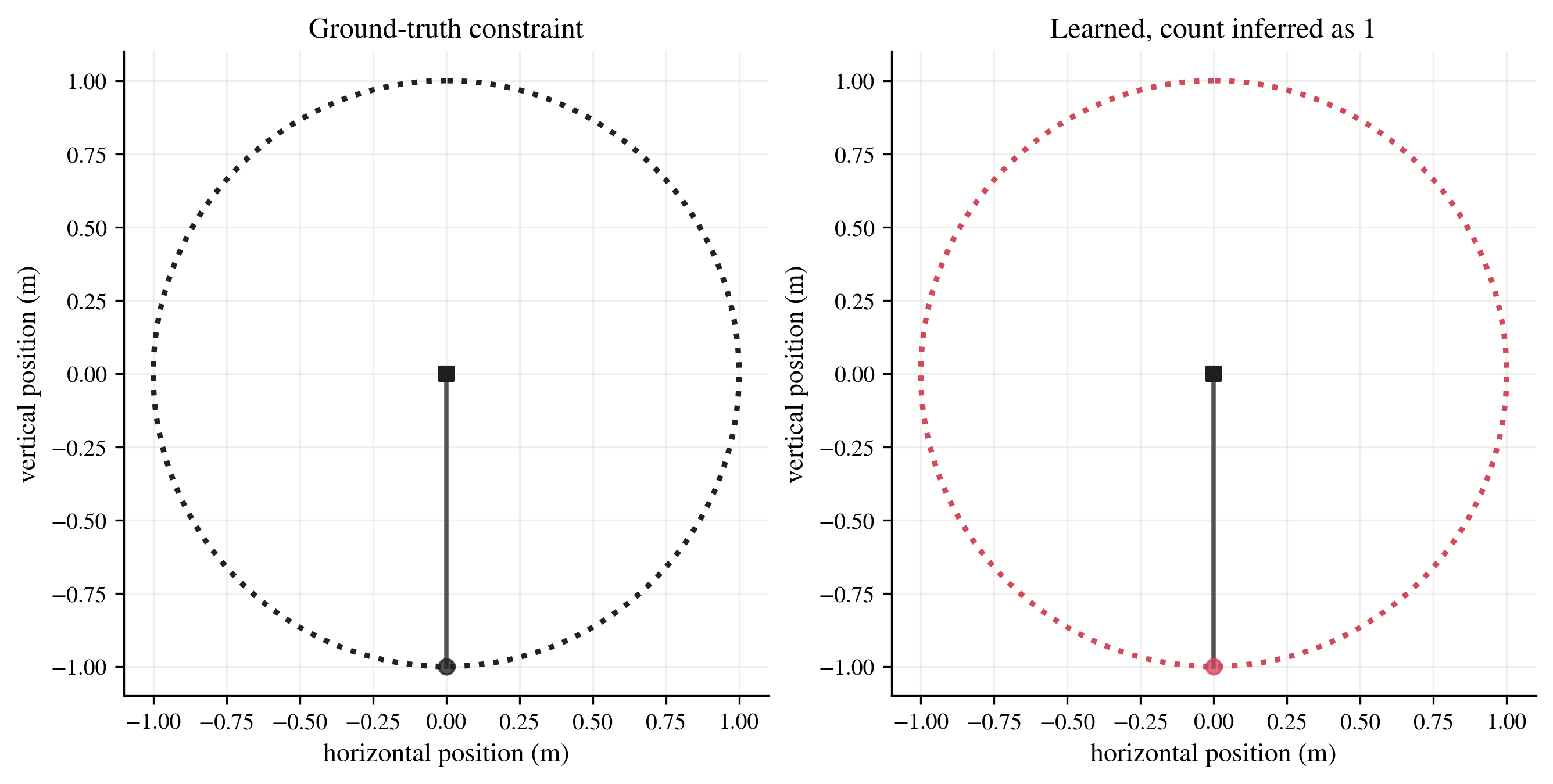
With these terms, the Lagrangian and constraint networks can train together for the single-pendulum system, and we recover the constraint pretty accurately.

The way to train these two networks together

Since the Lagrangian and constraint networks both affect each other’s gradient updates through very complicated signals, we need to be careful about how we train the system. The method we settled on is a three-stage training schedule:

1. Constraint first, freeze the LNN. The zero set alone already provides meaningful supervision for the constraint network, while a random Lagrangian would inject poor early signals.
2. Dynamics second, freeze the constraint network. The LNN can leave its random initialization without deforming the learned surface to compensate for bad dynamics.
3. Joint refinement, unfreeze both. Acceleration and geometry now provide complementary training signals to the two networks.

But this is still not enough for the general multidimensional case

For multidimensional systems, the constraint network can still be underconstrained. Let’s take the double pendulum as an example. We have the inputs $(x_{1},y_{1},x_{2},y_{2})$ for two point particles, so the unconstrained space is four-dimensional. Since we have two independent constraints, the normal space is two-dimensional. The tangent space, where our velocities live, is therefore

$$\underbrace{4}_{\text{ambient}} -\underbrace{2}_{\text{constraints}} =\underbrace{2}_{\text{tangent dimensions}}.$$

But our Jacobian loss term ensures only that the Jacobians are perpendicular to one particular velocity direction. One might hope that, on average, it would work during training, but in my experiments, it did not.

So, we need a method of estimating the tangent space. The method that I found to work is:

1. For a specific configuration, find nearby configurations. I used K-nearest neighbors.
2. Apply PCA to their velocities and extract the orthogonal directions with the highest velocity variance.
3. Penalize the non-orthogonality of the Jacobian with respect to all of these directions.

If $U_i$ contains the estimated local tangent directions, the multidirectional loss is

$$\mathcal L_{\rm tangent} =\mathbb E_i\,\|J_\psi(\mathbf q_i)U_i^\top\|_F^2.$$

With this method, I was successfully able to train the network for multidimensional systems such as the double pendulum.

How do we learn the number of constraints in the first place?

Until now, we have left an important part unexplored: how to infer the number of constraints. I did this using the same mechanisms we have just discussed:

1. Initialize the network to output the maximum possible number of constraints. Assuming zero degrees of freedom is not the case, this number is $n-1$.
2. Use the same KNN and PCA method and sort the PCA eigenvalues, which correspond to the variance along orthogonal directions in the tangent space.
3. Identify a large gap between the eigenvalues.
4. Count the number of eigenvalues before that gap to estimate the tangent-space dimension $\widehat d$.
5. Infer the number of constraints as $\widehat m=n-\widehat d$, and activate that many constraint outputs.

Then, I implicitly condition the network to output the inferred number of constraints as well.

Final results

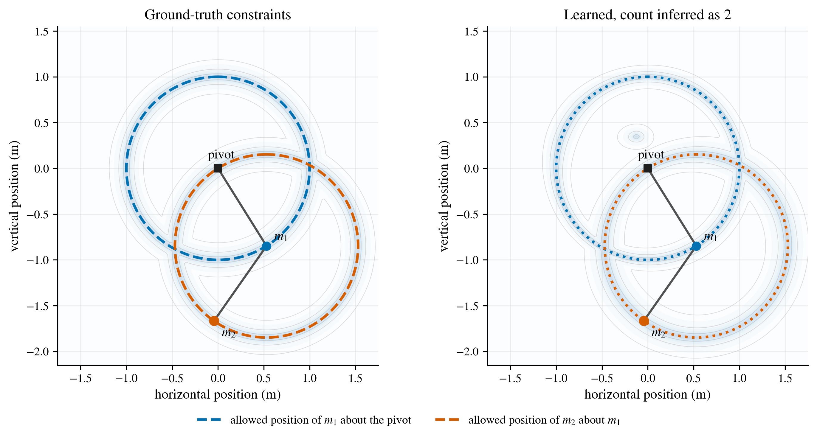
For the double pendulum, it predicted the dynamics really well, far exceeding the performance of LNNs with “good” coordinates, which kind of supports the claim that Lagrangians are simpler to learn in Cartesian coordinates.

Here are the learned constraints for a particular configuration of the double pendulum:

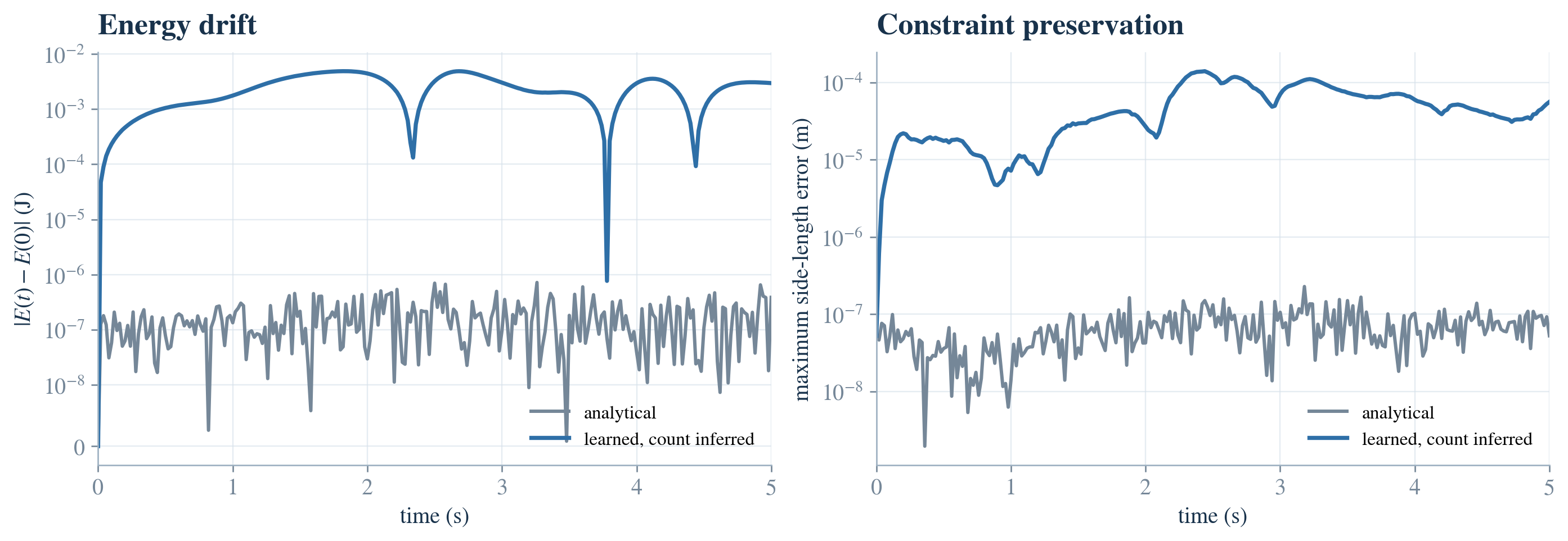
The other physical system for which we tried the framework is a rigid triangle. All corners have masses, one corner is linked to a spring, and gravity acts on every mass. Three fixed side lengths leave three degrees of freedom: two translations and one rotation.

Both the energy conservation and the constraint error are really good. The constraint error is defined as the largest change in the length of any rod at any time.

Conclusion

The framework successfully learns both the Lagrangian and the constraints, and inferring the number of constraints does not lead to a decrease in performance. Very exciting places to use this framework outside simple particle systems and robotics would include physical situations with gauge constraints, such as electromagnetism. I assume that the architecture would need to be modified, but now we have a very strong backbone to make something like this happen.

I also think it would be very fun to extend this to actual astrophysical data, since we no longer need to have good coordinates to use LNNs. But, of course, we also have to make sure that the framework has reasonable performance with sparse data.

Finally, as future work, inferring the number of constraints can be made more robust, since I observed it failing when I tried it on a zero-constraint system.

Bibliography

1. Lagrangian Neural Networks with Simultaneously Learned Constraints, EuCAIFCon 2026 presentation
2. Finzi, Wang, and Wilson, Simplifying Hamiltonian and Lagrangian Neural Networks via Explicit Constraints